Introduction to fastknn

The goal of fastknn is to make it easy for machine learning researchers and Kaggle competitors to create and tune KNN classifiers for very large datasets. It is based on the ANN library for fast nearest neighbor searching.

Getting Started

In this example fastknn is applied over a sample of size 50k from the Covertype dataset. It contains 54 binary variables and 7 possible class labels.

## Load packages
library("fastknn")
library("caTools")

## Load data
data("covertype", package = "fastknn")
x <- as.matrix(covertype[, -55])
y <- as.factor(covertype$Target)

## Split data for training and test
set.seed(123)
tr.idx <- which(caTools::sample.split(Y = y, SplitRatio = 0.7))
x.tr   <- x[tr.idx, ]
x.te   <- x[-tr.idx, ]
y.tr   <- y[tr.idx]
y.te   <- y[-tr.idx]

## Fit KNN
t1 <- system.time({
   knn.out <- fastknn(x.tr, y.tr, x.te, k = 15, method = "dist")
})
t1

user.self	sys.self	elapsed
0.516	0.004	0.519

Extremely fast!

Pre-Processing

The fastknn() function provides 4 options to normalize data before the nearest neighbors searching process:

normalize="std": standardize variables by removing the mean and scaling to unit variance.
normalize="minmax": transforms variables by scaling each one between 0 and 1.
normalize="maxabs": scales each variable by its maximum absolute value. This is the best choice for sparse data because it does not shift/center the variables.
normalize="robust": scales variables using statistics that are robust to outliers. It removes the median and scales by the interquartile range (IQR).

## Apply min-max normalization
knn.norm <- fastknn(x.tr, y.tr, x.te, k = 15, method = "dist", normalize = "minmax")

## Performance without normalization
sprintf("Logloss without normalization: %.3f", classLoss(y.te, prob = knn.out$prob, eval.metric = "logloss"))

## Performance with nromalization
sprintf("Logloss with normalization: %.3f", classLoss(y.te, prob = knn.norm$prob, eval.metric = "logloss"))

## [1] "Logloss without normalization: 0.507"

## [1] "Logloss with normalization: 0.611"

For this dataset, normalization had a negative effect on classification performance, but in many cases it is important to transform variables to the same unit before fitting KNN.

Find the Best k

The fastknn provides a n-fold cross-validation procedure to define the best k according to 4 different evaluation metrics:

"overall_error": overall misclassification rate
"mean_error": average in-class misclassification rate
"auc": average in-class area under the ROC curve
"logloss": cross-entropy error

cv.out <- fastknnCV(x, y, k = c(5, 10, 15), method = "dist", folds = 5, eval.metric = "overall_error")
cv.out$cv_table

fold_1	fold_2	fold_3	fold_4	fold_5	mean	k
0.1189	0.123	0.1274	0.1304	0.1207	0.1241	5
0.1329	0.1359	0.142	0.1388	0.1354	0.137	10
0.149	0.1548	0.1549	0.1529	0.1465	0.1516	15

Parallelization is available. You can specify the number of threads via nthread parameter.

Plot Decision Boundaries

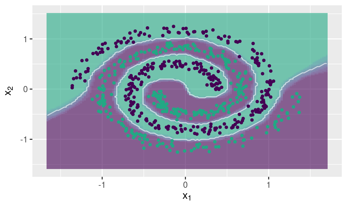
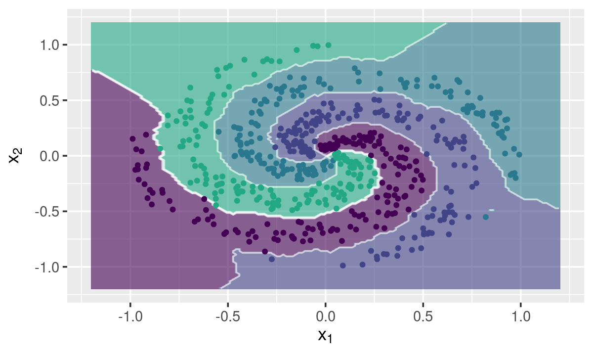
The fastknn provides a plotting function to draw classification decision boundaries for bi-dimensional datasets.

Two-class Toy Example

data("spirals", package = "fastknn")

## Split data for training and test
set.seed(123)
tr.idx <- which(caTools::sample.split(Y = spirals$y, SplitRatio = 0.7))
x.tr   <- spirals$x[tr.idx, ]
x.te   <- spirals$x[-tr.idx, ]
y.tr   <- spirals$y[tr.idx]
y.te   <- spirals$y[-tr.idx]

## Plot decision boudary
knnDecision(x.tr, y.tr, x.te, y.te, k = 10, method = "dist")

Multi-class Toy Example

data("multi_spirals", package = "fastknn")

## Split data for training and test
set.seed(123)
tr.idx <- which(caTools::sample.split(Y = multi_spirals$y, SplitRatio = 0.7))
x.tr   <- multi_spirals$x[tr.idx, ]
x.te   <- multi_spirals$x[-tr.idx, ]
y.tr   <- multi_spirals$y[tr.idx]
y.te   <- multi_spirals$y[-tr.idx]

## Plot decision boudary
knnDecision(x.tr, y.tr, x.te, y.te, k = 10, method = "dist")

Probability Estimation

The fastknn provides 2 different estimators to the class membership probabilities:

The classical estimator based on the label proportions of the nearest neighbors. This estimator can be thought as of a voting rule.
A shrinkage estimator based on the distances from the nearest neighbors, so that those neighbors more close to the test observation have more importance on predicting the class label. This estimator can be thought as of a weighted voting rule. In general, it reduces log-loss.

VOTING

#### 5-fold cross-validation
set.seed(123)
res <- fastknnCV(x, y, k = 10, method = "vote", folds = 5, eval.metric = "logloss")
res$cv_table

fold_1	fold_2	fold_3	fold_4	fold_5	mean	k
0.6081	0.5524	0.5643	0.5682	0.6528	0.5892	10

WEIGHTED VOTING

#### 5-fold cross-validation
set.seed(123)
res <- fastknnCV(x, y, k = 10, method = "dist", folds = 5, eval.metric = "logloss")
res$cv_table

fold_1	fold_2	fold_3	fold_4	fold_5	mean	k
0.5586	0.5039	0.5176	0.5181	0.604	0.5404	10

David Pinto