A Definitive Guide to Tune and Combine H2O Models in R
Building well-tuned H2O models with random hyper-parameter search and combining them using a stacking approach
This tutorial shows how to use random search (Bergstra and Bengio 2012) for hyper-parameter tuning in H2O models and how to combine the well-tuned models using the stacking / super learning framework (LeDell 2015).
We focus on generating level-one data for a multinomial classification dataset from a famous Kaggle challenge, the Otto Group Product Classification challenge. The dataset contains 61878 training instances and 144368 test instances on 93 numerical features. There are 9 categories for all data instances.
All experiments were conducted in a 64-bit Ubuntu 16.04.1 LTS machine with Intel Core i7-6700HQ 2.60GHz and 16GB RAM DDR4. We use R version 3.3.1 and h2o package version 3.10.0.9.
The source code and all output files are available on GitHub.
Repository Structure
When you are conducting a big experiment it’s very important to use a clear and robust repository structure, as follows:
root
│   README.md
│   project-name.Rproj
│
└── data
│   │  train.csv.zip
│   │  test.csv.zip
│   │  main.R
│   │...
│
└── gbm
│   │  main.R
│   │  gbm_output.csv.zip
│   │  gbm_model
│   │...
│
└── glm
│   │  main.R
│   │  glm_output.csv.zip
│   │  glm_model
│   │...
│
...
In the root directory we save a README.md file describing the experiment, and a RStudio project if we are using the RStudio IDE (strong recommended). In the data folder we save the data files and a R script to read them to the memory. Then we create a separated folder for each machine learning algorithm, where we store the R scripts to run it and the generated outputs like predictions and fitted models.
Split Data in k-Folds
The first step is to split data in folds. We will use k-fold cross-validation for parameter tuning and then to generate level-one data to be used in the stacking step. All algorithms will use the same fold ids. So, we generate them using the caret package and save the results in the ./data/ folder. Here we use k = 5.
We have fixed the random generator with set.seed(2020) to allow reproducibility.
## Load required packages
library("readr")
library("caret")

## Read training data
tr.data <- readr::read_csv("./data/train.csv.zip")
y <- factor(tr.data$target, levels = paste("Class", 1:9, sep = "_"))

## Create stratified data folds
nfolds <- 5
set.seed(2020)
folds.id <- caret::createFolds(y, k = nfolds, list = FALSE)
set.seed(2020)
folds.list <- caret::createFolds(y, k = nfolds, list = TRUE)
save("folds.id", "folds.list", file = "./data/cv_folds.rda",
     compress = "bzip2")
Import Data to H2O
## Load required packages
library("h2o")
library("magrittr")

## Instantiate H2O cluster
h2o.init(max_mem_size = '8G', nthreads = 6)
h2o.removeAll()

## Load training and test data
label.name <- 'target'
train.hex <- h2o.importFile(
   path = normalizePath("./data/train.csv.zip"),
   destination_frame = 'train_hex'
)
train.hex[,label.name] <- h2o.asfactor(train.hex[,label.name])
test.hex <- h2o.importFile(
   path = normalizePath("./data/test.csv.zip"),
   destination_frame = 'test_hex'
)
input.names <- h2o.colnames(train.hex) %>% setdiff(c('id', label.name))

## Assign data folds
load('./data/cv_folds.rda')
train.hex <- h2o.cbind(train.hex, as.h2o(data.frame('cv' = folds.id),
                                         destination_frame = 'fold_idx'))
h2o.colnames(train.hex)
Tuning GBM
For more details about GBM parameters take a look at this tutorial Complete Guide to Parameter Tuning in Gradient Boosting (GBM) in Python. There is also a great tutorial showing how to build a well-tuned H2O GBM model, the H2O GBM Tuning Tutorial for R.
Random Parameter Search
## Random search for parameter tuning
gbm.params <- list(
   max_depth = seq(2, 24, by = 2),
   min_rows = seq(10, 150, by = 10),                 # minimum observations required in a terminal node or leaf
   sample_rate = seq(0.1, 1, by = 0.1),              # row sample rate per tree (boostrap = 0.632)
   col_sample_rate = seq(0.1, 1, by = 0.1),          # column sample rate per split
   col_sample_rate_per_tree = seq(0.1, 1, by = 0.1),
   nbins = round(2 ^ seq(2, 6, length = 15)),        # number of levels for numerical features discretization
   histogram_type = c("UniformAdaptive", "Random", "QuantilesGlobal", "RoundRobin")
)
gbm.grid <- h2o.grid(
   algorithm = "gbm", grid_id = "gbm_grid",
   x = input.names, y = label.name, training_frame = train.hex,
   fold_column = "cv", distribution = "multinomial", ntrees = 500,
   learn_rate = 0.1, learn_rate_annealing = 0.995,
   stopping_rounds = 2, stopping_metric = 'logloss', stopping_tolerance = 1e-5,
   score_each_iteration = FALSE, score_tree_interval = 10,
   keep_cross_validation_predictions = TRUE,
   seed = 2020, max_runtime_secs = 30 * 60,
   search_criteria = list(
      strategy = "RandomDiscrete", max_models = 25,
      max_runtime_secs = 12 * 60 * 60, seed = 2020
   ),
   hyper_params = gbm.params
)
Select the Best Parameters
## Get best model
grid.table <- h2o.getGrid("gbm_grid", sort_by = "logloss", decreasing = FALSE)@summary_table
save(grid.table, file = "./gbm/grid_table.rda", compress = "bzip2")
best.gbm <- h2o.getModel(grid.table$model_ids[1])
h2o.logloss(best.gbm@model$cross_validation_metrics)
h2o.saveModel(best.gbm, path = "./gbm", force = TRUE)
file.rename(from = paste("gbm", grid.table$model_ids[1], sep = "/"), to = "gbm/best_model")
best.params <- best.gbm@allparameters
save(best.params, file = "./gbm/best_params.rda", compress = "bzip2")

head(grid.table, 5)
| col_sample_rate | col_sample_rate_per_tree | histogram_type | max_depth | min_rows | nbins | sample_rate | model_ids | logloss |
|---|---|---|---|---|---|---|---|---|
| 1.0 | 0.5 | RoundRobin | 14 | 70.0 | 35 | 0.8 | gbm_grid_model_6 | 0.4643 |
| 0.3 | 0.7 | Random | 22 | 50.0 | 35 | 0.6 | gbm_grid_model_15 | 0.4649 |
| 0.6 | 0.4 | RoundRobin | 10 | 70.0 | 24 | 1.0 | gbm_grid_model_10 | 0.4767 |
| 0.8 | 1.0 | UniformAdaptive | 24 | 60.0 | 35 | 0.4 | gbm_grid_model_28 | 0.4792 |
| 1.0 | 0.8 | RoundRobin | 22 | 140.0 | 9 | 0.4 | gbm_grid_model_14 | 0.4847 |
Generate Level-one Training Data
## Get predictions for the training cv folds
var.names <- paste("gbm", 1:h2o.nlevels(train.hex[,label.name]), sep = "_")
gbm.train.hex <- h2o.getFrame(best.gbm@model$cross_validation_holdout_predictions_frame_id$name)
gbm.train.hex[,"predict"] <- NULL
colnames(gbm.train.hex) <- var.names
gbm.train.hex <- h2o.round(gbm.train.hex, 6)
gbm.train.hex <- h2o.cbind(gbm.train.hex, train.hex[,label.name])
write.csv(
   as.data.frame(gbm.train.hex),
   file = gzfile('./gbm/gbm_levone_train.csv.gz'),
   row.names = FALSE
)
Generate Level-one Test Data
## Get predictions for the test set
gbm.test.hex <- predict(best.gbm, test.hex)
gbm.test.hex[,"predict"] <- NULL
gbm.test.hex <- h2o.round(gbm.test.hex, 6)
write.csv(
   as.data.frame(gbm.test.hex),
   file = gzfile('./gbm/gbm_levone_test.csv.gz'),
   col.names = var.names,
   row.names = FALSE
)
Generate Test Predictions
## Save output for the test set
gbm.out.hex <- h2o.cbind(test.hex[,"id"], gbm.test.hex)
write.csv(
   as.data.frame(gbm.out.hex),
   file = gzfile('./gbm/gbm_output.csv.gz'),
   row.names = FALSE
)
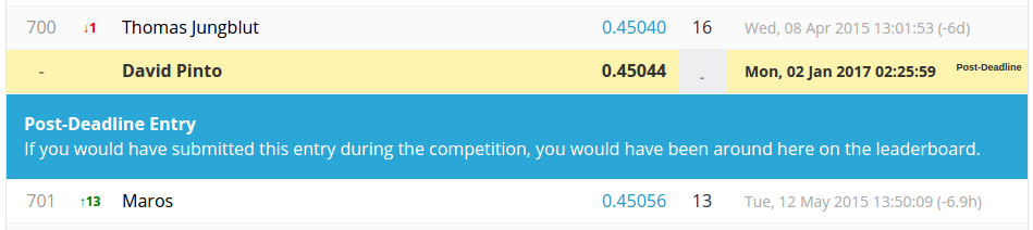
Top 20% with a single GBM model.
Tuning RandomForest
…
Tuning DeepLearning
…
Tuning GLM
…
Tuning NaiveBayes
…
Super Learner
The approach presented here allow you to combine H2O with other powerful machine learning libraries in R like XGBoost, MXNet, FastKNN, and caret, through the level-one data in the .csv format. You can also use the level-one data with Python libraries like scikit-learn and Keras.
We recommed the R package h2oEnsemble as an alternative to easily build stacked models with H2O algorithms.
References
Bergstra, James, and Yoshua Bengio. 2012. “Random Search for Hyper-Parameter Optimization.” Journal of Machine Learning Research 13 (February): 281–305.
LeDell, Erin. 2015. “Intro to Practical Ensemble Learning.” University of California, Berkeley.